

- The influence of three PID parameters in sulfuric acid production on the control curve
In sulfuric acid production, PID serves as a primary control strategy widely applied across various control systems. It comprises the controlled object, measurement and transmission components, feedback controllers, and end-effectors. However, in practical operations, many find PID tuning daunting, primarily due to unfamiliarity with the essence of the three PID parameters and their impact on control curves.
This paper aims to explain PID concepts in clear and concise language. It uses simulation curves to detail how the three PID parameters specifically affect the tuning curve in sulfuric acid chemical production.
1. Limitations of the threshold judgment method
Controlling the five major chemical parameters—temperature, pressure, liquid level, composition, and flow rate—is essential in actual sulfuric acid production. Taking temperature control as an example, the simplest approach without any control algorithm is threshold judgment: immediately halting heating measures when temperature exceeds a setpoint. Under ideal safe production conditions, this yields a control curve:
微信截圖_20251024105318_20251024.png)
Figure 1.1 Simulation fitting curve under threshold control
The simulation results reveal irregular fluctuations. Factors such as the sensitivity of control components and heating performance may cause oscillations, making effective control challenging. In sulfuric acid production, high temperatures combined with transmitter lag and thermal conduction delays prevent threshold control from responding promptly, potentially amplifying vibrations. This is where PID control demonstrates its advantages. PID stands for "Proportion Integration Differentiation," essentially a formula comprising three components: the proportional term (Proportion), the integral term (Integration), and the derivative term (Differentiation). Its specific form is as follows:
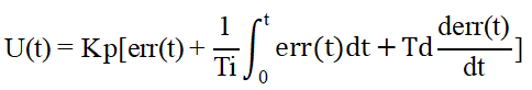
U(t) represents the output control variable;
Kp denotes the proportional gain;
Ti denotes the integral time;
Td denotes the derivative time constant;
err(t) denotes the error, which is the difference between the setpoint (SV) and the process variable (PV).
1.1 Proportional gain Kp
As shown in the formula, it is evident that without integral and derivative actions, the PID kp value exhibits a linear relationship with the output signal. Suppose the output control variable (valve opening) ranges from 20% to 70%, and the input error (err) ranges from 50 to 100°C. When err is 50°C, the output must reach 20%. The proportional coefficient establishes this linear relationship between input and output. For Kp, a higher value increases proportional action, accelerating response speed and reducing error. However, excessively high proportional gain can cause oscillations, degrading system stability. The comparison diagram below visually illustrates the phenomena that occur as proportional gain increases.
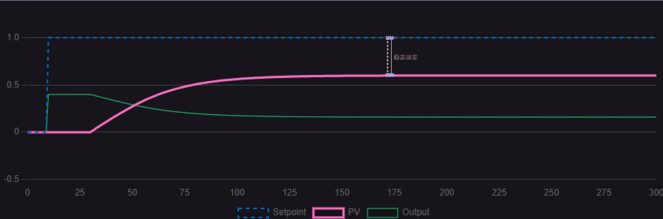
Figure 1.1.1 The proportional gain of Kp is 1
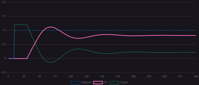
Figure 1.1.2 The proportional gain of Kp is 3
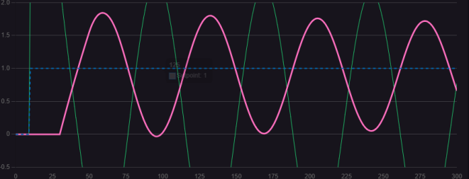
Figure 1.1.3 The proportional gain of Kp is 5.7
Comparing the three control curves, an appropriate Kp value effectively accelerates response speed and eliminates steady-state error. An excessively low Kp value causes significant steady-state error, while an excessively high Kp value results in oscillation with constant amplitude.
1.2 Integration Time Ti
Control curves with only proportional gain show no significant difference from the threshold judgment method mentioned earlier. In fact, excessively small or large proportional gains perform worse than the threshold judgment method. Building upon this, integral and derivative control are introduced. The integral coefficient corresponds to the area under the control curve, representing the cumulative error over the corresponding time period. By multiplying this accumulated value by a coefficient and applying it to the output, steady-state error can be partially eliminated, enhancing system stability. The integral time is inversely proportional to the integral effect. Next, we will present and analyze the control curve with integral action incorporating proportional action, exploring the specific role of integral action within the control curve.
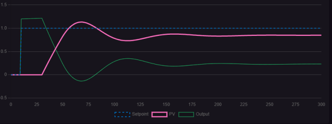
Figure 1.2.1 Control Curve graph when P=3 and I=0.002
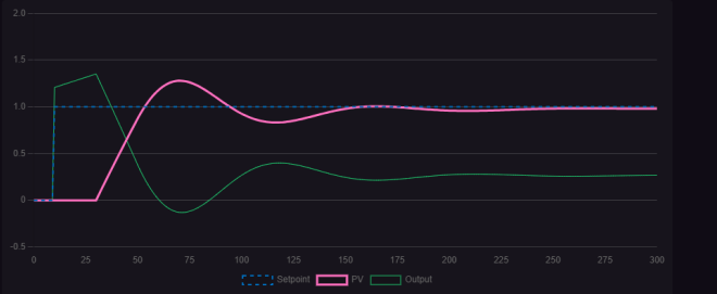
Figure 1.2.2 Control Curve graph when P=3 and I=0.018
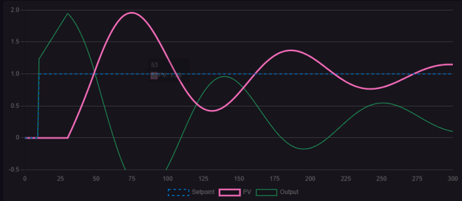
Figure 1.2.3 Control Curve graph when P= 3I=0.089
Observing the three figures, compared to control curves with only proportional gain, a small amount of integral action has some effect on eliminating steady-state error, though not significantly. As the integral action increases, the control curve gradually converges with the target line, and the steady-state error is essentially eliminated. However, further increasing the integral action causes noticeable damped oscillations with prolonged duration, though the waveform ultimately converges toward the target value. Thus, integral action effectively eliminates steady-state error, but excessive integral action slows dynamic response and induces long-period damped oscillations. In practical control processes, process variable (PV) fluctuations within a certain range are permissible. Selecting an appropriate proportional action can accelerate the regulation speed, but it will be accompanied by a certain amount of overshoot. It is necessary to ensure that this overshoot is within the allowable range of production errors to achieve stable, accurate, and fast response of the control system. Figure 1.2.4 shows the control curve under appropriate proportional action.
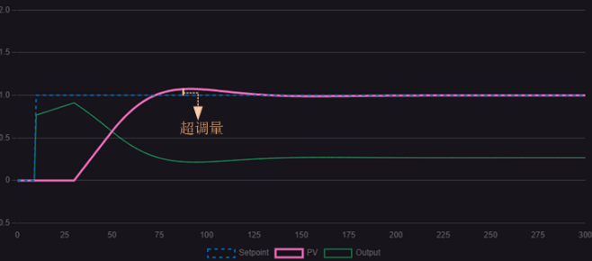
Figure1.2.4 P=3 I=0.019
1.3 Differential Time Td
The purpose of the derivative action is to reduce overshoot and shorten the settling time. This will be explained in detail below using simulation curves.
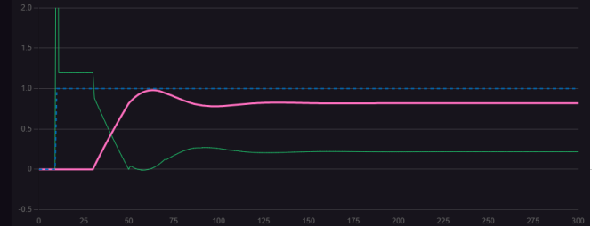
Figure1.3.1 P=3 D=12.5
Comparing Figures 1.1.2 and 1.3.1, the addition of derivative action significantly reduces overshoot and oscillation amplitude while shortening the time required to reach steady-state
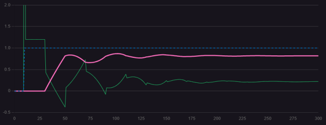
Figure1.3.2 P=3 D=40
Increasing the derivative term significantly reduces overshoot. However, improper derivative action can cause oscillations in the control curve, prolonging the stabilization time and potentially making system stability difficult to achieve.
Neither derivative nor integral action can control independently, nor can they operate in isolation; both require proportional action to function effectively.
1.4 PID System Regulation
First, perform parameter tuning based on the PI system: adjust the proportional coefficient P first, then the integral coefficient I. This ensures the system exhibits appropriate overshoot while rapidly reaching steady state. Simultaneously, ensure the error remains within acceptable limits without affecting subsequent processes or triggering interlock mechanisms. Specific simulation results are shown below:
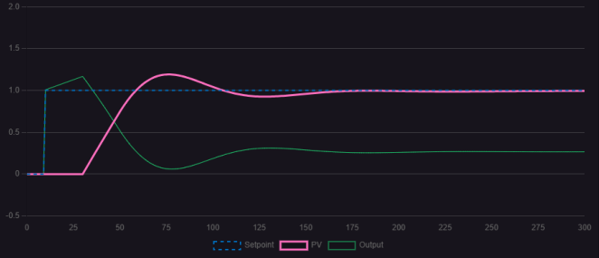
Figure 1.4.1 Tuning curve under PI action
Gradually introduce derivative action to eliminate overshoot and further reduce settling time, as shown below:
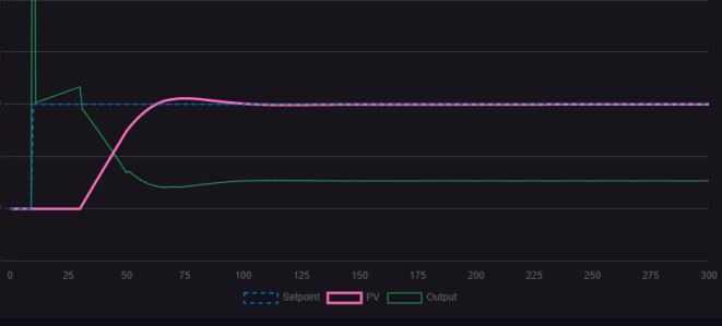
Figure 1.4.2 Tuning curve under PID action
The figure above demonstrates that the curve obtained through PID control is relatively smoother. However, in practical control applications, both types of actions are typically combined. As long as the error remains within permissible limits and does not significantly impact production, PI control is generally adopted. It is noteworthy that PI control accounts for as much as 75% of applications across the entire chemical engineering field.
Kp, Ti, and Td interact with each other, and the tuning process is time-consuming, making perfect control quite challenging. This paper only briefly analyzes the debugging approach. Factors to consider in actual operation are more complex, including controller selection, mutual interference between single closed loops, and the inertia and lag effects of the control system.